May 2017
Random Forests
Or how to grow a forest of random Decision Trees with scikit-learn
Random Forests are a popular example of an Ensemble Learning method. Ensemble Learning consists on combining multiple machine learning (ML) models in order to achieve higher predictive performance than could be obtained using either of the individual models alone. Ensemble Learning methods work best when the models are as diverse as possible, providing complementary predictive performance. One way to achieve this is to combine models built using different ML algorithms, to leverage their diverse strengths. An alternative approach is to use the same ML algorithm, but to train each model on a different random subset of the training data. This is the appproach taken by Random Forests: they combine multiple Decision Tree models trained on random subsets of the training data.
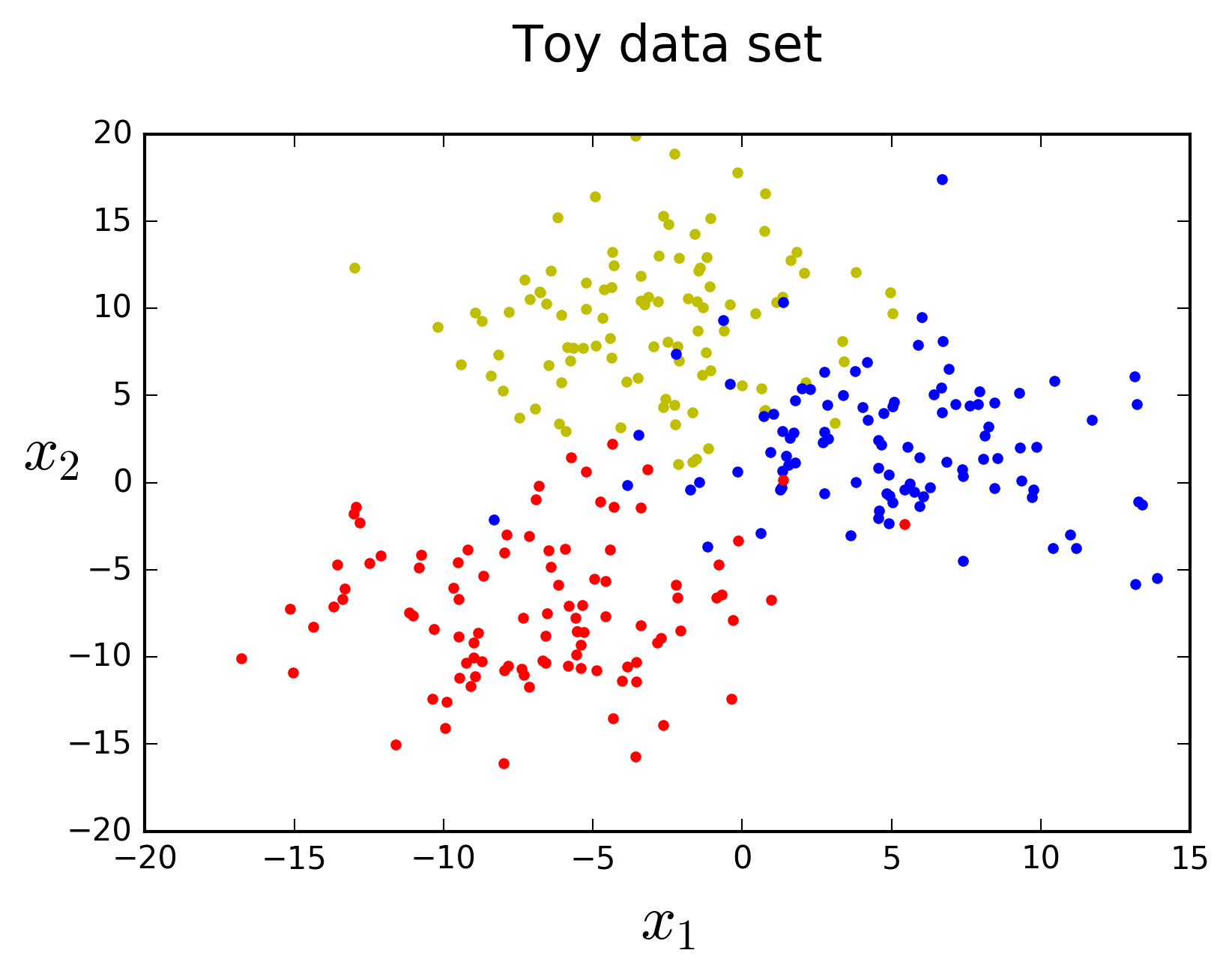
In this post I will start by taking a closer look at the Decision Tree ML algorithm and then discuss how you can combine different Decision Tree models to build Random Forests. Before moving on, let's generate some toy data using scikit-learn's
import matplotlib.pyplot as plt

# Generate data
from sklearn.datasets import make_blobs
X, y = make_blobs(n_samples=300, n_features=2, centers=3,
                  cluster_std=4, random_state=42)

# Plot data
plt.plot(X[:, 0][y==0], X[:, 1][y==0], "yo", marker='.')
plt.plot(X[:, 0][y==1], X[:, 1][y==1], "bs", marker='.')
plt.plot(X[:, 0][y==2], X[:, 1][y==2], "rd", marker='.')
plt.xlabel(r"$x_1$", fontsize=20)
plt.ylabel(r"$x_2$", fontsize=20, rotation=0)
plt.title("Toy data set\n", fontsize=16)
1. Decision Trees
1.1 Making predictions
Decision Trees are powerful ML algorithms capable of fitting complex data sets. The Wikipedia page on Decision Tree Learning presents the following definition:
A decision tree is a flow-chart-like structure, where each internal (non-leaf) node denotes a test on an attribute, each branch represents the outcome of a test, and each leaf (or terminal) node holds a class label. The topmost node in a tree is the root node.
In order to classify a data instance, all you need to do is traverse the flow chart, answering all the tests, until you reach a leaf node. Each test will be a question conerning a specific feature in the data. The class labeling of the leaf node the new instance ends up in is the predicted class. Let's grow a Decision Tree on our data to take a closer look at how this works in practice. scikit-learn makes this ridiculously easy, of course.
from sklearn.tree import DecisionTreeClassifier

# Instantiate the classifier class
tree_clf = DecisionTreeClassifier(max_depth=2, random_state=42)

# Grow a Decision Tree
tree_clf.fit(X, y)
We have grown a tree on our 2-D data set. Classifying new observations is simple. Let's make up a couple of examples to try the classifier on.
import numpy as np

# Define function to classify observations
def predict_class(data_point, classes=['Yellow', 'Blue', 'Red']):
    # Convert to appropriate numpy array
    data_point = np.array(data_point).reshape(1, -1)

    # Classify
    result = tree_clf.predict(data_point)

    # Print output
    print('Predicted class for point {}: {}'.format(data_point,
                                                    classes[np.asscalar(result)]))

# Classify some example observations
predict_class([-5, 10])
predict_class([10, 5])
predict_class([-10, -10])
Predicted class for point [[-5 10]]: Yellow
Predicted class for point [[10  5]]: Blue
Predicted class for point [[-10 -10]]: Red
If you check the location of the points visually in the plot above you will see that these predictions make sense. Let's visualize the Decision Tree model to inspect its structure and see how it makes decisions. We can use the
from sklearn.tree import export_graphviz

export_graphviz(tree_clf, out_file='tree.dot',
                feature_names=['x1', 'x2'],
                class_names=['Yellow', 'Blue', 'Red'],
                rounded=True, filled=True)
We can then convert the
dot -Tpng tree.dot -o tree.png
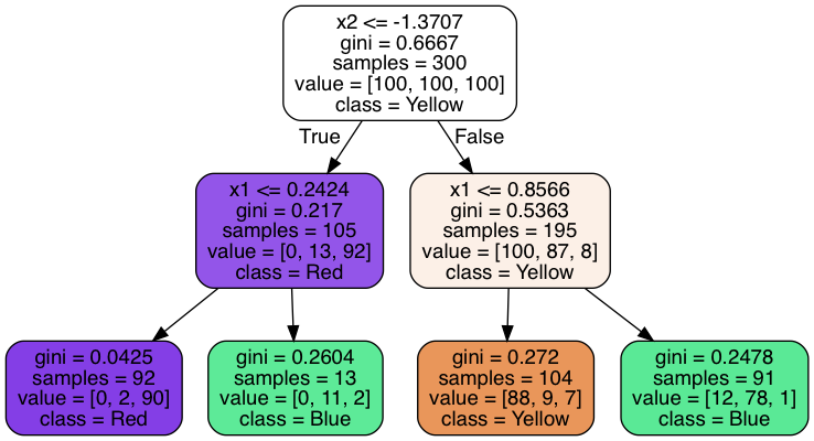
We can now see the exact way the model predicts new instance classes. At the root node we find all 300 training examples split evenly between the three classes. The tree asks whether the value of feature \(x2\) is lower than or equal to \(−1.3707\). It splits the data in two groups according to the answer and then goes on to ask another question in each of the two following internal nodes. These, in turn, split the data between two groups each. Since we set argument
Let's use one of the instances predicted above as an example: \(x1=−5, x2=10\). The answer to the root node question is
This structure allows Decision Trees to estimate class probabilities by simply computing the ratio of training instances belonging to each class in the leaf node. For example, for our predicted instance above this tree estimates it belongs to class "Yellow" with 84.6% probability (88/104; the predicted class), class "Blue" with 8.7% probability (9/104) and class "Red" with 6.7% probability (7/104).
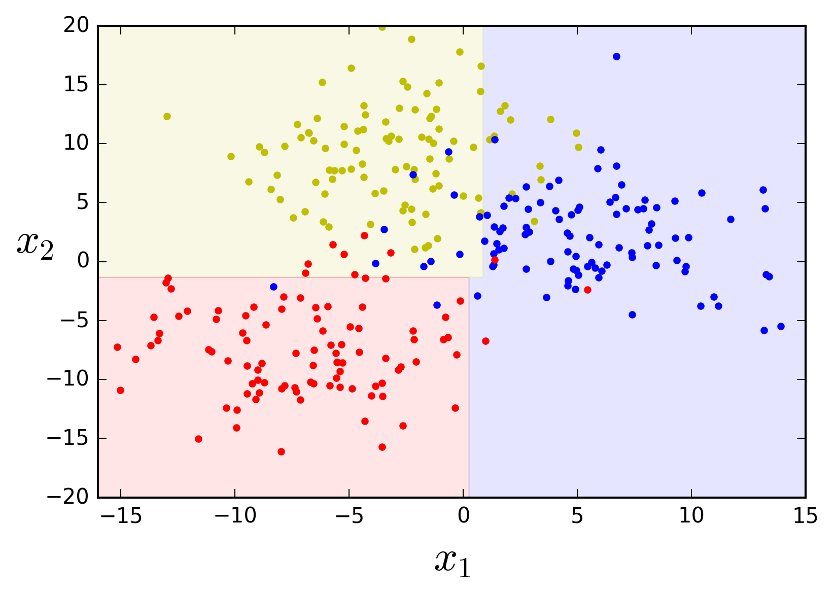
These rules define axis-parallel decision boundaries, dividing the feature space into a series rectangles, each of which predicts only one of the classes. Let's define a function to compute the decision boundaries and a function to plot them, together with the training data, using matplotlib.
from matplotlib.colors import listedcolormap

def compute_decision_boundaries(clf, x, y, axes):
    x1s = np.linspace(axes[0], axes[1], 300)
    x2s = np.linspace(axes[2], axes[3], 300)
    x1, x2 = np.meshgrid(x1s, x2s)
    x_new = np.c_[x1.ravel(), x2.ravel()]
    y_pred = clf.predict(x_new).reshape(x1.shape)

    return x1, x2, y_pred

def plot_feature_space(clf, x, y, axes, file_name=none):
    x1, x2, y_pred = compute_decision_boundaries(clf, x, y, axes)
    custom_cmap = listedcolormap(['y','b','r'])
    plt.contourf(x1, x2, y_pred, cmap=custom_cmap, alpha=0.1, linewidth=1)
    plt.plot(x[:, 0][y==0], x[:, 1][y==0], "yo", marker='.')
    plt.plot(x[:, 0][y==1], x[:, 1][y==1], "bs", marker='.')
    plt.plot(x[:, 0][y==2], x[:, 1][y==2], "rd", marker='.')
    plt.axis(axes)
    plt.xlabel(r"$x_1$", fontsize=20)
    plt.ylabel(r"$x_2$", fontsize=20, rotation=0)
    if file_name is not none:
        plt.savefig(file_name, dpi=300, bbox_inches='tight')
    plt.figure(figsize=(8, 4))
Now we can plot the decison space for this example.
plot_feature_space(tree_clf, X, y, axes=[-16, 15, -20, 20])
1.2 "Growing" a Decision Tree model
So this is how a Decision Tree model makes predictions. But how can we actually grow the tree? There are alternatives, but scikit-learn uses the Classification And Regression Tree (CART) algorithm. CART works by splitting the training set of \(m\) instances into two subsets using a single feature \(k\) and a threshold \(t_k\), such that the split produces the purest subsets (weighted by their size). This is called the splitting rule. It then splits the subsets in the same exact way, then the sub-subsets and so on, recursively, until it cannot find a split to reduce class impurity. This is known as constructing the maximum tree. The CART algorithm minimizes the following cost function at each split:
$$ J(k, t_k) = \dfrac{m_{left}}{m}I_{left} + \dfrac{m_{right}}{m}I_{right} $$ $$ with \begin{cases} I_{left/right} \text{ impurity of the left/right subset,}\\ m_{left/right} \text{ number of instances in the left/right subset.} \end{cases} $$So what is the impurity \(I\) measure? Typically, this will be the Gini impurity. Formally:
$$ I_G(t) = 1 - \sum_{k=1}^K p_{k,t}^2 $$ $$ with \begin{cases} k \bbox[3pt]{1, . . . , K} \text{ index of the class,}\\ p_{k,t} \text{ ratio of class $k$ instances among the training instances in node $t$} \end{cases} $$In other words, the Gini impurity measures the probability that a randomly chosen instance from the node would be incorrectly labeled if it were randomly labeled according to the distribution of classes in the node. It does this by first computing the probability \(p_{k,t}\) that a randomly chosen instance from the subset of training instances in the node \(t\) belongs to class \(k\) (simply the ratio of class \(k\) instances). It multiplies this probability by itself, which yields the probability \(p_{k,t}^2\) that that instance would be correctly labeled if it were randomly labeled according to the distribution of classes in the node (again, simply the ratio of class \(k\) instances). It then sums up the probabilities across all classes \(K\) and finally computes the probability that the instance would be incorrectly classified by subtracting the previous probability from the unity. The Gini impurity is thus reduced to zero when the node is pure, i.e. all instances in the node belong to the same class, since in that case \(p_{k,t} = 1\) for the represented class (and 0 for all others) and thus \(p_{k,t}^2 = 1\), resulting in \(I_G(t) = 1 - 1 = 0\).
You can now go back to the image of the tree structure and check the "gini" attribute at each node. Let's take, for example, the purple leaf node \(t=4\). Using the definition above, we can calculate the Gini impurity at this is node and get the indicated value of \(0.0425\):
$$ I_G(4) = 1 - \sum_{k=1}^K p_{k,4}^2 = \\ = 1 - \left( {\left(\dfrac{0}{92}\right)}^2 + {\left(\dfrac{2}{92}\right)}^2 + {\left(\dfrac{90}{92}\right)}^2 \right) =\\ = 1 - ( 0 + 0.00047 + 0.95699 ) =\\ = 0.0425 $$This is quite a pure node, since 97.8% of the observations belong to the same class ("Red"). It corresponds to the lower left section of the decision space plot above. Its Gini impurity measure is consequently very low. An alternative to Gini impurity is to use the Information gain measure, based on the concept of entropy from information theory. In scikit-learn you can use this measure by instantiating the
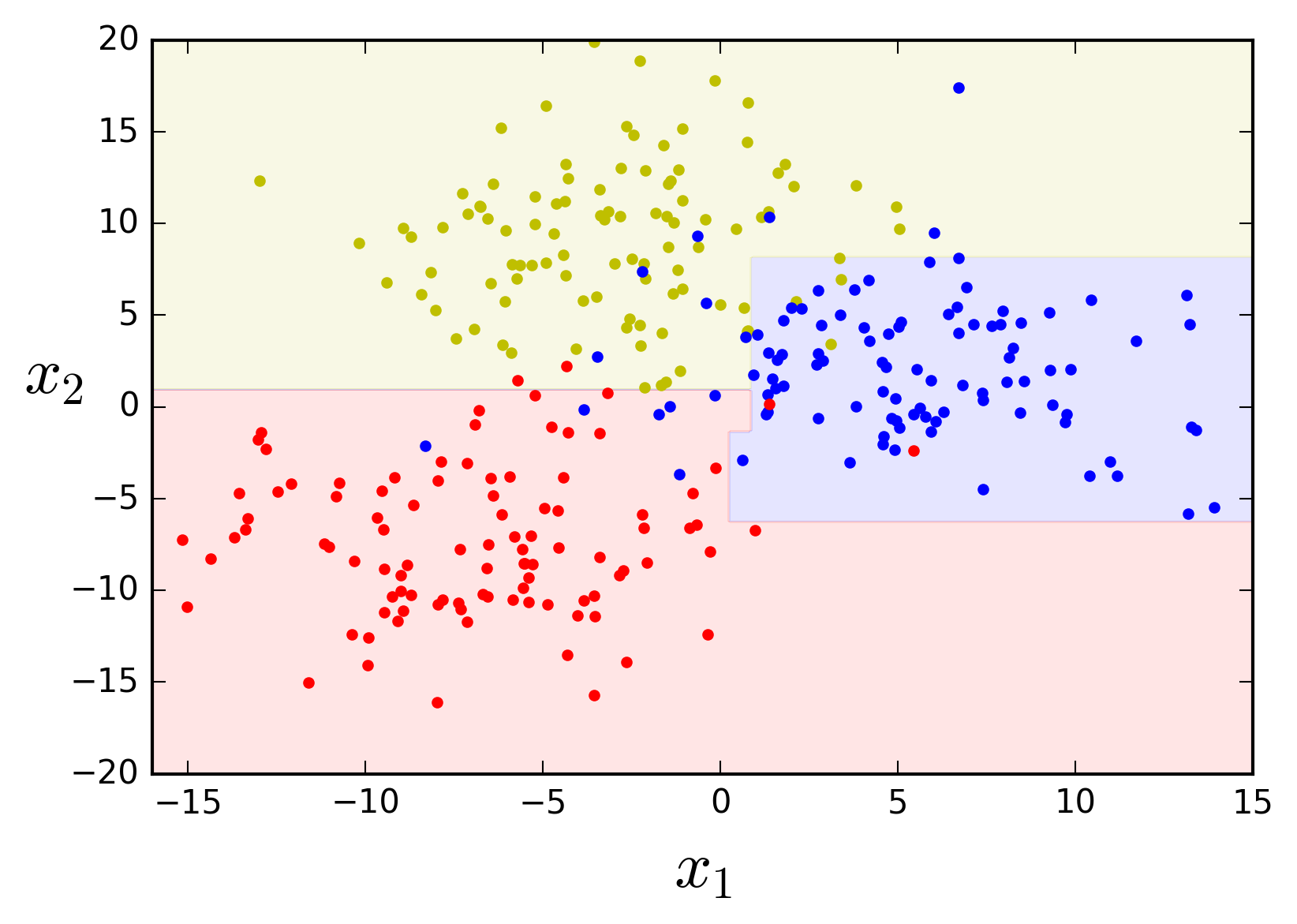
Decision Trees have the ability to adapt very closely to the training data. They are non-parametric models, since the number of parameters is not predetermined and will thus grow during training. This means that they have a tendency to produce high-variance models that will not generalize well to classification of new, previously unseen, instances. This is known as overfitting the training data. For this reason, regularization is very important when training Decision Tree models. Decision Trees have several regularization hyperparameters. Different implementations will, at the very least, allow you to constrain the tree depth. You may have noticed that I have used that above, by instantiating the
# Instantiate the classifier class for a deeper tree
tree_clf = DecisionTreeClassifier(max_depth=3, random_state=42)

# Grow a Decision Tree
tree_clf.fit(X, y)

plot_feature_space(tree_clf, X, y, axes=[-16, 15, -20, 20])
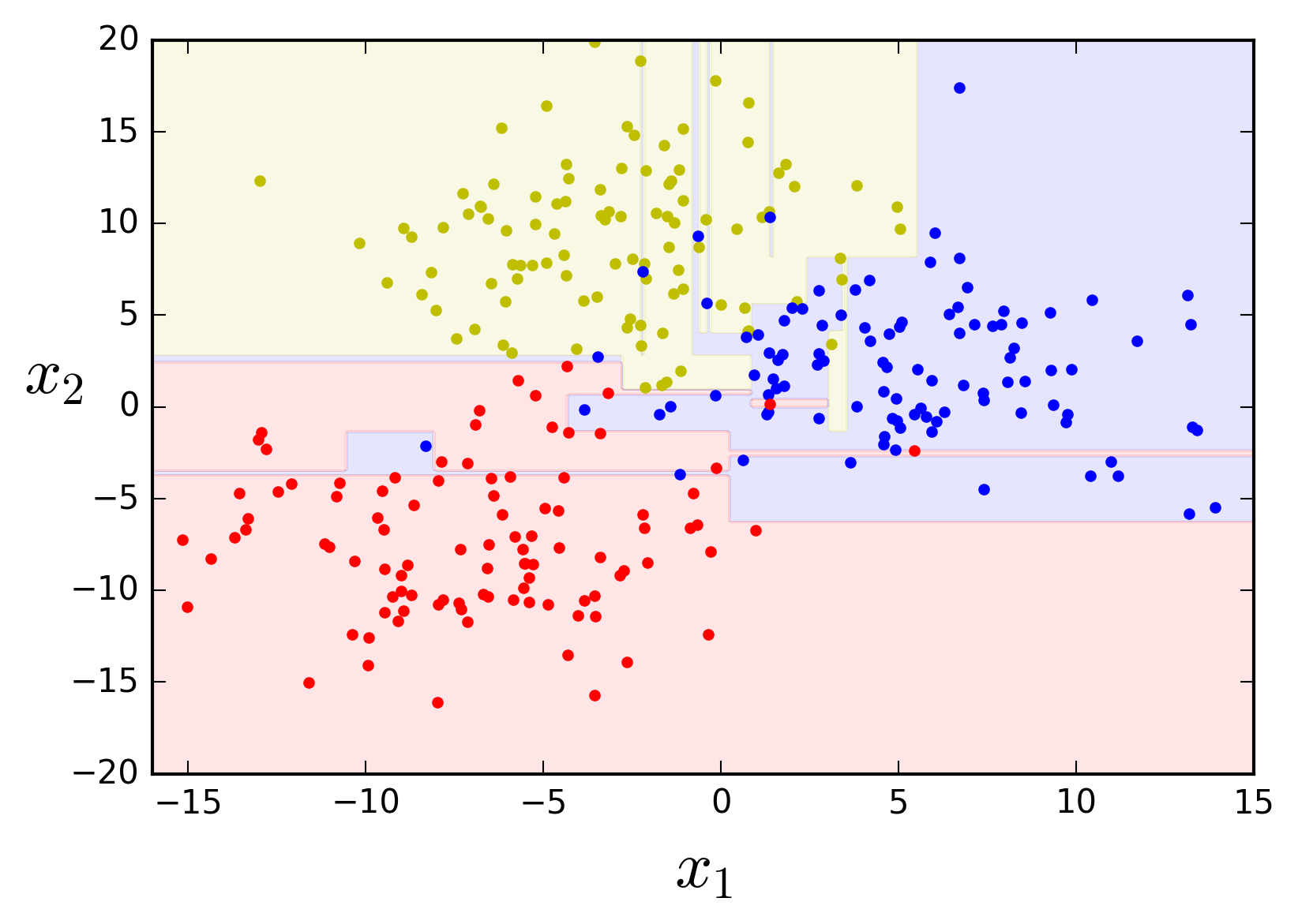
If left unconstrained the algorithm tries hard to fit the data, learning every single data point's class and thus producing an overcomplicated model.
# Instantiate the classifier class with no limits
tree_clf = DecisionTreeClassifier(random_state=42)

# Grow a Decision Tree
tree_clf.fit(X, y)

plot_feature_space(tree_clf, X, y, axes=[-16, 15, -20, 20])
Additional regularization parameters provided by scikit-learn include the minimum number of instances in a node before it can be split, the minimum number of instances in a leaf node, the maximum number of leaf nodes, and the maximum number of features that are evaluated for each split.
Decision Trees can also be used for regression problems, instead of classification, with very minor changes. The tree is grown in the same way, using the CART algorithm, except that instead of minimizing node impurity it minimizes the mean squared error (MSE). It then simply predicts the average value of all data observations at each node, instead of the most common class.
2. Random Forests
2.1 Building an ensemble of Decision Trees
An ensemble of Decision Trees is called a Random Forest. Random Forests are an example of ensemble modeling using the same ML algorithm to build multiple models each trained on a different random subset of the training data. When the training data sampling for each predictor is performed with replacement, the method is called Boosted aggregating, commonly abbreviated to Bagging. Sampling without replacement is called Pasting. After growing the Random Forest, i.e. training the chosen number of Decision Trees, the individual Decision Trees vote to reach the final prediction. Voting can be done in two ways, called hard voting and soft voting. Hard voting consists on using the statistical mode of the predicted classes, i.e. the most commonly predicted class. Soft voting consists on outputing the highest class probability, averaged over all the individual classifiers. This, of course, requires that the predictors be able to estimate class probabilities.
The final result is typically a model with similar bias but a lower variance than a single Decision Tree trained on the same data. This means that the decision boundary is less irregular. Let's see what that looks like by using scikit-kearn's
from sklearn.ensemble import BaggingClassifier

bag_clf = BaggingClassifier(DecisionTreeClassifier(), n_estimators=50,
                            max_samples=50, bootstrap=True, n_jobs=-1,
                            oob_score=True, random_state=42)

bag_clf.fit(X, y)

plot_feature_space(bag_clf, X, y, axes=[-16, 15, -20, 20])
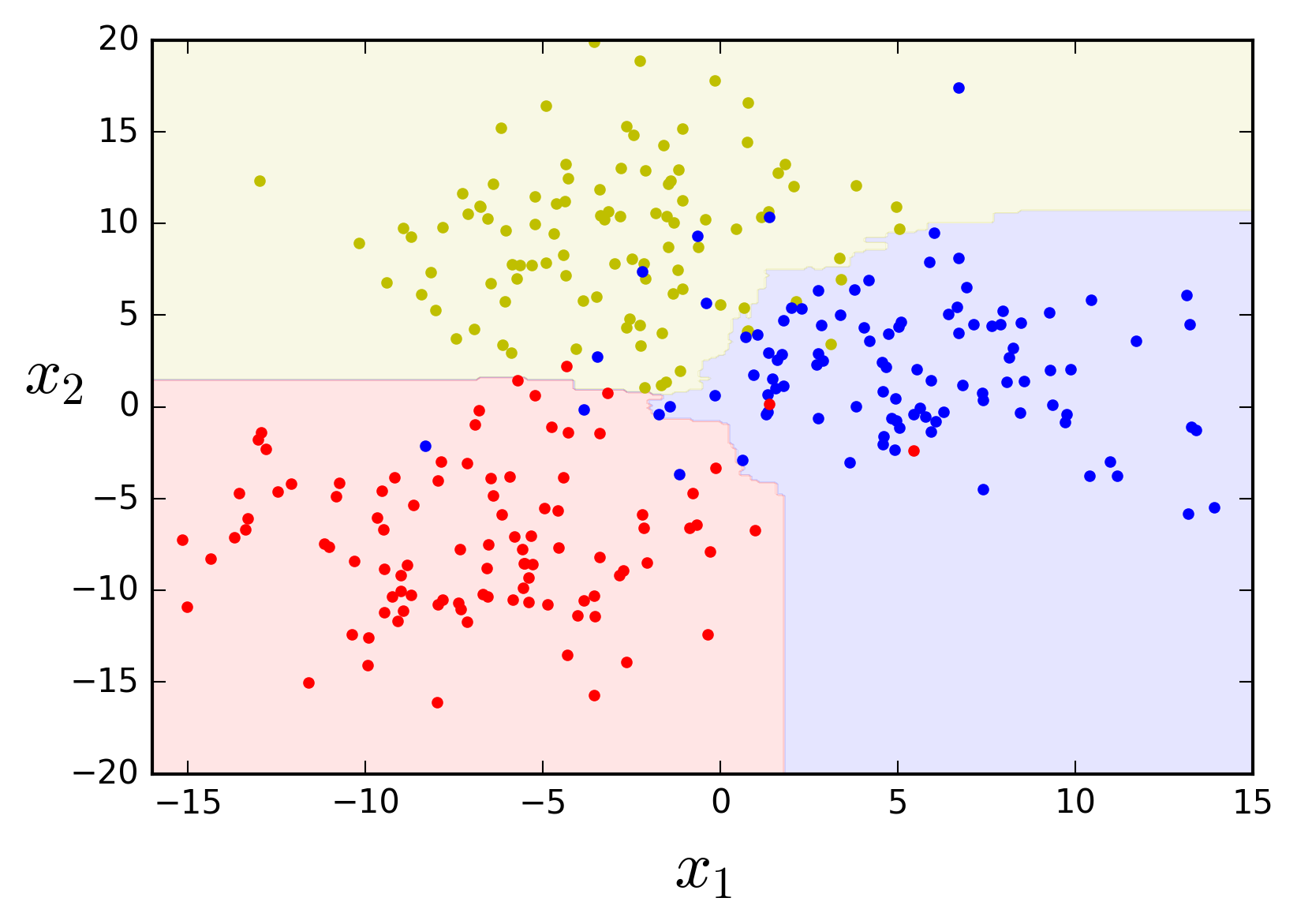
The decision boundaries look much smoother and definitely seem like they will generalize much better. An interesting side-effect of the bagging procedure is that a subset of the instances will not be sampled during training, the so-called out-of-bag instances. The model will not have seen the out-of-bag instances at all during training and so they can actually be used as a test set, in a procedure known as Out-of-bag Evaluation. Parameter
print('Out-of-bag evaluation score: {}%'.format(round(bag_clf.oob_score_, 4) * 100))
Out-of-bag evaluation score: 91.0%2.2 The Random Forest Classifier class
As you may know, scikit-learn actually has a
from sklearn.ensemble import RandomForestClassifier

rf_clf = RandomForestClassifier(n_estimators=50, max_leaf_nodes=10, n_jobs=-1,
                                bootstrap=True, oob_score=True, random_state=42)

rf_clf.fit(X, y)

plot_feature_space(rf_clf, X, y, axes=[-16, 15, -20, 20])
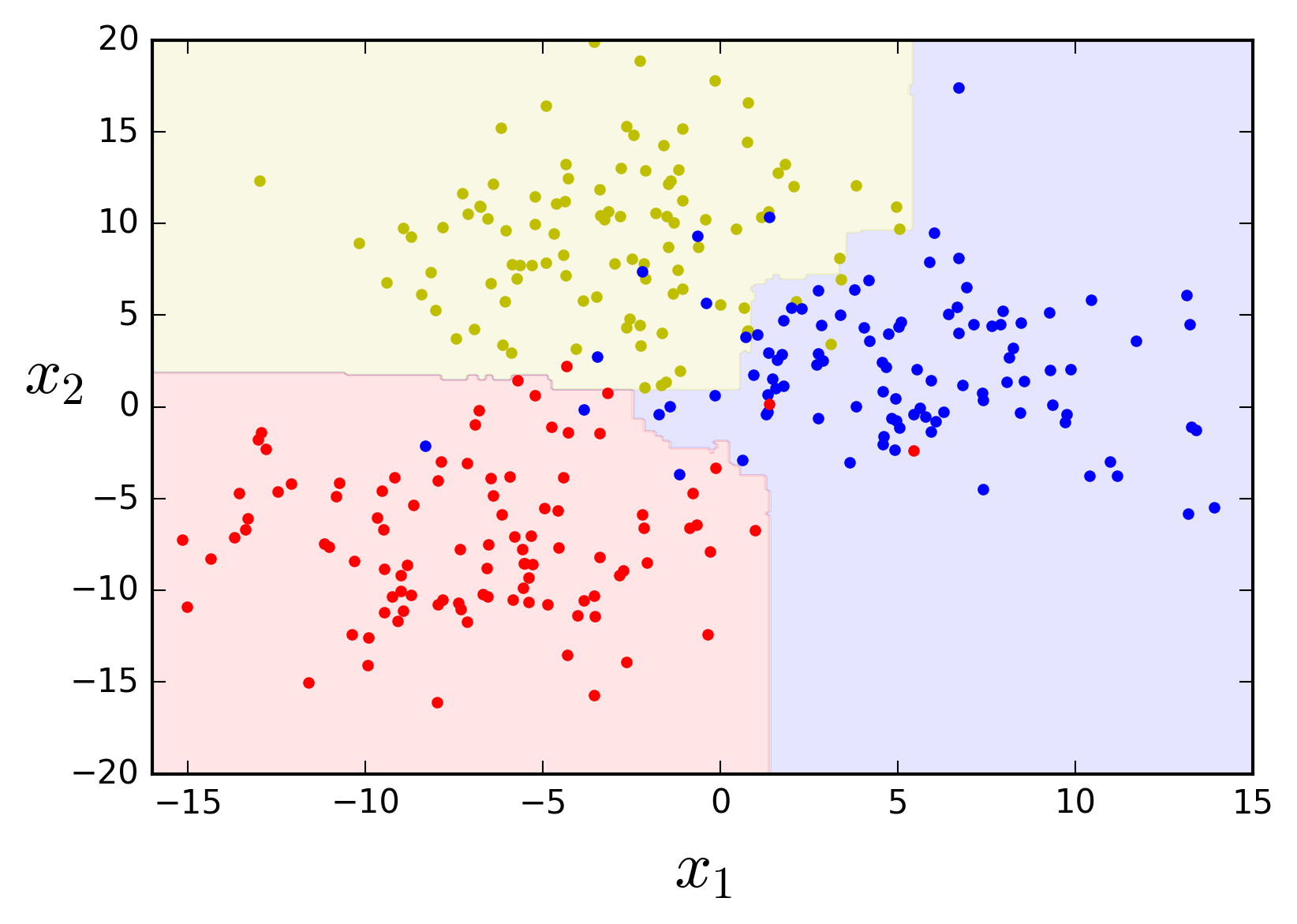
print('Out-of-bag evaluation score: {}%'.format(round(rf_clf.oob_score_, 4) * 100))
Out-of-bag evaluation score: 91.33%3. Extremely Randomized Trees
There is yet another tree-based ensemble algorithm implementation in scikit-learn introducing additional randomness: the Extremely Randomized Trees ensemble or Extra-Trees. Besides considering only a subset of the data set at each node, the Extra-Tree algorithm uses random splitting thresholds for each feature, rather than searching for the best threshold, to make its Decision Tree predictors even more random. Here's what it looks like with our toy data.
from sklearn.ensemble import ExtraTreesClassifier

extra_clf = ExtraTreesClassifier(n_estimators=50, max_leaf_nodes=10, n_jobs=-1,
                                 bootstrap=True, oob_score=True, random_state=42)

extra_clf.fit(X, y)

plot_feature_space(extra_clf, X, y, axes=[-16, 15, -20, 20])
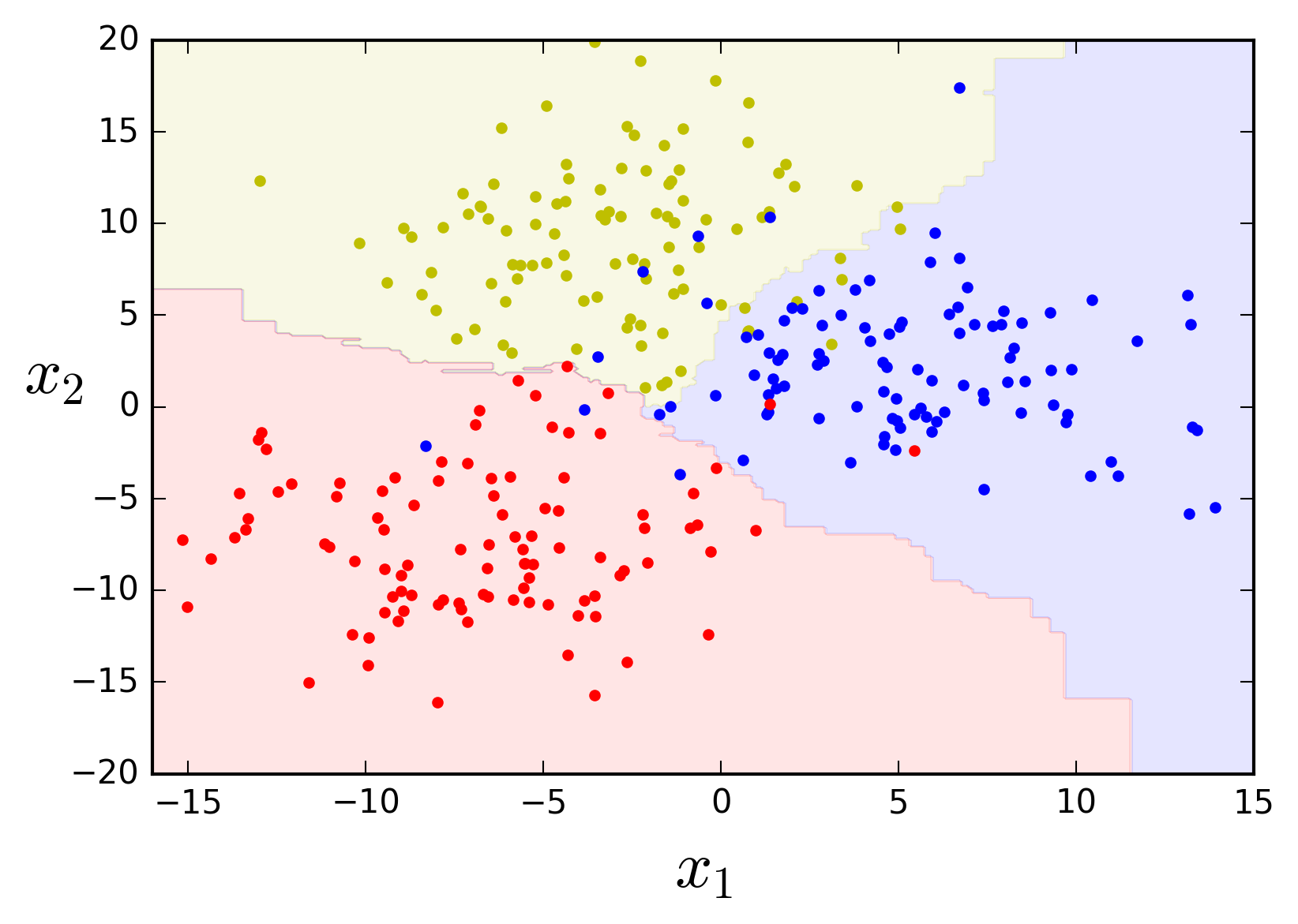
print('Out-of-bag evaluation score: {}%'.format(round(extra_clf.oob_score_, 4) * 100))
Out-of-bag evaluation score: 92.0%The decision boundaries look even more natural, right?
That's it for this overview of Random Forests. I hope this helped you get a deeper understanding of Decision Trees, Ensemble Learning, and Random Forests.